Note on Weinberg's textbooks on QFT

Notation. The Latin indices such as

, etc., typically span the three spatial coordinate labels, commonly denoted as 1, 2, 3. On the other hand, Greek indices like

, and so forth, usually range over the four spacetime coordinate labels, specifically 1, 2, 3, 0, where

represents the time coordinate. Indices that appear twice are usually summed unless specified otherwise. The spacetime metric, denoted by

, is a diagonal matrix with elements

and

. The d'Alembertian is represented as

and defined by the equation

, where

is the Laplacian given by

. The ‘ Levi-Civita tensor,’ symbolized by

, is an entirely antisymmetric entity with

. Spatial vectors in three dimensions are marked by boldface characters. A unit vector corresponding to any vector is shown with a hat, as in

. A dot over a variable signifies its time derivative. The Dirac matrices

adhere to

, and

, while

. The step function

yields a value of +1 when

and 0 when

. For a matrix or vector

, the complex conjugate, transpose, and Hermitian adjoint are represented by

, and

respectively. The Hermitian adjoint of an operator

is marked as

, except when an asterisk emphasizes that a vector or matrix of operators is not transposed. Terms like +H.c. or +c.c. appended to equations indicate the addition of the Hermitian adjoint or complex conjugate of preceding terms. A Dirac spinor

with a bar over it is defined as

. Apart from in Chapter ?, units are normalized such that

and the speed of light are set to one. The fine structure constant is represented as

, calculated as

, approximately

, where

is the rationalized charge of the electron. Parenthetical numbers next to quoted numerical figures signify the uncertainty in the last digits. Unless otherwise stated, experimental data is sourced from ‘Review of Particle Properties,’ Phys. Rev. D50, 1173 (1994).

The perspective presented argues that quantum field theory exists in its current form due to its unique capability to harmonize quantum mechanics with special relativity, under some conditions. Our initial endeavor is to explore how symmetries, such as Lorentz invariance, manifest within a quantum context in the following aspects.

Quantum field theory rests on the same foundational quantum mechanics developed by Schrödinger, Heisenberg, Pauli, Born, and other pioneers in 1925–1926.

A symmetry transformation can be thought of as a shift in perspective that does not affect the outcomes of potential experiments. If an observer

perceives a system in a state denoted by a ray

..., a corresponding observer

scrutinizing the same system would view it in a different state, symbolized by a ray

..., respectively. However, both observers must ascertain the same probabilities:

This condition is necessary but not sufficient for a ray transformation to qualify as a symmetry; additional conditions will be elaborated upon in the following chapter. Wigner proved a significant theorem in the early 1930s, stating that for any such transformation

, an operator

can be defined in the Hilbert space. If

is a vector in ray

, then

belongs to ray

. The operator

can either be unitary and linear:

This finding is called the fundamental theorem of Wigner and the proof is the following:

for all rays and ; and vectors , , , and . Then there exists an operator acting on such that

for all ray and all ; and that either is unitary and linear or antiunitary and antilinear.

This definition does not apply to an antilinear operator since the right-hand side of (1.2.6) would be linear in

, while the left-hand side is antilinear in

. For an antilinear operator

, the adjoint is instead specified as:

Given this definition, the criteria for either unitarity or antiunitarity can both be expressed as:

There exists a trivial symmetry transformation ℛ→ℛ, represented by the identity operator

. This operator is naturally unitary and linear. Continuity dictates that any symmetry operation (like a rotation, translation, or Lorentz transformation) that can be reduced to a trivial transformation by continuously adjusting certain parameters (such as angles, distances, or velocities) must be characterized by a linear unitary operator

, as opposed to one that is antilinear and antiunitary. (Symmetries represented by antiunitary antilinear operators are less common in physics; they all entail a reversal in the direction of time flow. See Section ? for more details.)

Specifically, a symmetry transformation that is nearly trivial on an infinitesimal scale can be depicted by a linear unitary operator that is infinitesimally close to the identity operator:

Here,

is a real infinitesimal. For

to be both unitary and linear,

needs to be Hermitian and linear, making it a potential observable. In fact, many (if not all) physical observables, like angular momentum or momentum, are derived from symmetry transformations in this manner.

The set of symmetry transformations possesses specific characteristics that categorize it as a group. If

is a transformation converting rays

, and

is another transformation that maps

, then the outcome of executing both transformations consecutively is yet another symmetry transformation, denoted as

, that transforms

into

. Additionally, any symmetry transformation

that changes

into

has an inverse, expressed as

, which reverts

back to

. Moreover, there exists an identity transformation,

, which leaves rays unaltered.

The unitary or antiunitary operators

that correspond to these symmetry transformations emulate this group structure, albeit with added complexity because

operators act on vectors in Hilbert space instead of on rays. If

transforms

into

, then applying

to a vector

must result in a vector

. If

then maps this ray to

must also belong to

, as must

. Therefore, the vectors can only differ by a phase factor

, as given by:

Moreover, barring a notable exception, the linearity (or antilinearity) of

specifies that these phases are state-independent. To prove this, let us consider two non-proportional vectors

and

and apply Equation (1.2.10) to the state:

Every unitary or antiunitary operator has an inverse (its adjoint), which is also either unitary or antiunitary. Upon left-multiplying Equation (1.2.11) by

, we arrive at:

Consequently, the phase in Equation (1.2.10) is state-independent, leading to the operator relation:

When

, this indicates that

constitutes a representation of the group of symmetry transformations. For arbitrary phases

, we refer to it as a ‘projective representation’ or a representation ‘up to a phase’. Whether the Lie group structure allows for state vectors to furnish an ordinary or projective representation can not be inferred from the group structure alone but will become apparent later.

The exception to the reasoning that concluded in Equation (1.2.14) lies in the possibility that the system may not be preparable in a state represented by

. For example, it is generally considered unfeasible to prepare a system in a superposition of states with total angular momenta that are integers and half-integers. In such scenarios, we refer to the presence of a ‘superselection rule’ between different categories of states. As a result, the phases

could be contingent on which class of states the operators

and

are acting upon. Further details about these phases and projective representations will be discussed in Section ?. It will be shown that any symmetry group featuring projective representations can be extended (without altering its physical meaning) to allow for all its representations to be non-projective, i.e., with

. Until we reach Section ?, we will proceed with the assumption that such an extension has been applied, and will take

in (1.2.14). Also, the existence of spinor is partially derived from the phase ambiguity that arises when taking absolute values and the fact that the homotopy class of the homogeneous Lorentz group.

In physics, a specific type of group known as a connected Lie group holds special significance. These are groups comprised of transformations

, defined by a finite collection of real, continuous parameters, symbolized as

. Each group element is linked to the identity element through a continuous path within the group itself. The multiplication rule for the group is expressed as

where

is a function of both

and

. If

denotes the coordinates of the identity, then

must hold true. In the case of such continuous groups, the transformations must be represented in the physical Hilbert space by unitary operators

, rather than antiunitary ones. These unitary operators, at least in a finite vicinity of the identity, can be expressed by a power series as

Here,

, and so on, are Hermitian operators independent of

. Assuming that

provides a standard (non-projective) representation of the transformation group, meaning

we can expand this in terms of

and

. In accordance with Equation (1.2.16), the second-order expansion of

should be

Here,

are real coefficients. Note that the presence of any

terms would be in conflict with Equation (1.2.16). Following this, Equation (1.2.18) can be articulated as:

On both sides of Equation (1.2.20), terms of order 1,

, and

correspond without issue. However, when focusing on the

terms, a non-trivial condition emerges:

This reveals that if we know the group structure, specifically the function

and its corresponding quadratic coefficient

, we can determine the second-order terms of

using the first-order generators

. However, there's a requirement for consistency: the operator

has to be symmetric in

and

, as it's the second derivative of

with respect to

and

. Therefore, Equation (1.2.21) necessitates that

This kind of commutation relationship is termed a Lie algebra. In a later section, we will essentially demonstrate that this commutation relation (1.2.22) is the sole condition needed to perpetuate this computation. In other words, the complete power series for

can be generated from an endless chain of equations like Equation (1.2.21), as long as we are aware of the first-order terms, namely the generators

. While this does not mean

operators are uniquely identified for all

based solely on

, it does signify that they are uniquely specified within a finite vicinity of the identity coordinate

, such that Equation (1.2.15) holds true if

and

lie within this region. The discussion about extending this to all

will take place in a subsequent section.

There is a particular scenario of considerable relevance that will recur frequently in our discussions. Assume the function

is simply additive for some or all of the coordinates

, as expressed by:

This situation is applicable, for example, in the context of spacetime translations or for rotations about a single fixed axis (but not for both simultaneously). In this special case, the coefficients

from Equation (1.2.19) become zero, and likewise, the structure constants in Equation (1.2.23) also vanish. Consequently, the generators are commutative, denoted by:

Such a group is termed as Abelian. Under these conditions, computing

for all

becomes straightforward. According to Equations (1.2.18) and (1.2.24), for any integer

, we can express:

By taking the limit as

approaches infinity and retaining only the first-order term in

, we obtain:

Einstein's principle of relativity asserts the equivalence of specific 'inertial' frames of reference, setting it apart from the Galilean principle of relativity adhered to by Newtonian mechanics. The distinction comes from the transformation equations that link coordinate systems across different inertial frames. Given that

represents the coordinates in one inertial frame—where

are Cartesian spatial coordinates and

is a time coordinate (assuming the speed of light equals one)—the coordinates

in another inertial frame must satisfy:

The summation convention applies: any index like

and

in Equation (1.3.2) appearing twice, once as a superscript and once as a subscript, is summed over.

These transformations have the unique feature that the speed of light remains consistent—in our chosen units, equal to one—across all inertial frames. A light wave with unit speed satisfies

, or in terms of the equation

, which also implies

and thus

Here,

are arbitrary constants, and

is a constant matrix that meets the criteria:

For certain applications, it's advantageous to express the Lorentz transformation condition using an alternate formulation. The matrix

possesses an inverse, designated as

, which coincidentally has the same diagonal components:

and

These transformations constitute a group. When we initially apply a Lorentz transformation as per Eq. (1.3.4), and then follow it with another Lorentz transformation

, such that

we find that the overall transformation effect is identical to performing a Lorentz transformation

as described by

Here, it's worth noting that if

and

both meet the conditions of Eq. (1.3.5),

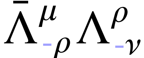will also be a Lorentz transformation. The bar notation is simply used to distinguish one Lorentz transformation from another. Correspondingly, the transformations

on physical states obey the composition law

This implies that

has an inverse, denoted as

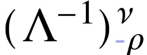, which as per Eq. (1.3.5) takes the form

According to Eq. (1.3.8), the inverse of the transformation

turns out to be

, and naturally, the identity transformation is represented by

Based on the dialogue in the prior section, the transformations

give rise to a unitary linear transformation acting on vectors in the physical Hilbert space, represented as

. These operators

obey a composition law articulated as

It's worth noting that to prevent the emergence of a phase factor on the right-hand side of Eq. (1.3.11), it's generally required to extend the Lorentz group. The suitable extension for accomplishing this is discussed in Section ?.

The complete set of transformations

is formally referred to as the inhomogeneous Lorentz group, also known as the Poincaré group. This group has several significant subgroups. First, transformations with

naturally constitute a subgroup, described by

which is termed the homogeneous Lorentz group. Additionally, from Eq. (1.3.9), it's evident that

can be either

; transformations having

inherently make up a subgroup of either the homogeneous or inhomogeneous Lorentz groups. Further scrutiny of the 00-components of Eqs. (1.3.5) and (1.3.6) yields

where

ranges over 1, 2, and 3. This shows that either

. Transformations where

constitute a subgroup. Observe that if

and

are two such matrices

, then

According to Eq. (1.3.13), the three-vector

has a length of

, and similarly, the three-vector

has a length of

. Therefore, the scalar product of these two three-vectors has an upper limit given by

This subgroup, characterized by

and

, is identified as the proper orthochronous Lorentz group. As one cannot smoothly transition from

, or from

, any Lorentz transformation derived from the identity through a continuous variation of parameters must share the same sign for

and

as the identity, and thus must be a member of the proper orthochronous Lorentz group.

Every Lorentz transformation falls into one of two categories: it is either proper and orthochronous, or it can be expressed as the composition of an element from the proper orthochronous Lorentz group and one of the discrete transformations

. Here,

represents the space inversion, which has non-zero elements given by

Therefore, a comprehensive understanding of the entire Lorentz group can be achieved by studying its proper orthochronous subgroup, along with the concepts of space inversion and time-reversal. The exploration of space inversion and time-reversal will be carried out separately in Section ?. Until that point, our focus will remain on either the homogeneous or inhomogeneous proper orthochronous Lorentz group.

As discussed in Section 1.2, many essential attributes of any Lie symmetry group are encapsulated in the properties of the elements in the vicinity of the identity element. In the context of the inhomogeneous Lorentz group, the identity transformation is given by

and

. Therefore, we aim to explore transformations that can be written as

where both

and

are infinitesimal. The Lorentz condition, expressed as equation (1.3.5), can be rewritten as

In this book, we adopt the convention that indices can be raised or lowered by contracting with

If we retain only the first-order terms in

in the Lorentz condition (1.3.5), we find that this condition simplifies to the antisymmetry of

An antisymmetric second-rank tensor in four dimensions has

independent components. Coupled with the four components of

, an inhomogeneous Lorentz transformation is thus characterized by

parameters.

Because

maps any ray onto itself, it must be proportional to the unit operator, and by a choice of phase may be made equal to it. Excluding the presence of superselection rules, we can eliminate the chance that this proportionality factor varies depending on the state acted upon by

. This exclusion follows the same logic we applied in Section 1.2 to dismiss the idea that phases in projective representations of symmetry groups might depend on the states they act upon. In cases where superselection rules are relevant, it could be necessary to adjust the phase factors of

depending on the sector it acts on.

For an infinitesimal Lorentz transformation as described by equation (1.4.1),

must be equal to the unit operator

augmented by terms that are linear in

and

. We express this relationship as

In this equation,

and

are operators that are independent of

and

, and the ellipsis signifies terms of higher order in

and/or

. For

to be unitary, operators

and

must be Hermitian:

(Yes, the generators of boosts are observables.) Given that

is antisymmetric, its coefficient

can also be taken to be antisymmetric:

As we will elaborate on later,

, and

are the components of the momentum operators;

, and

are the angular momentum vector components; and

is the energy operator or Hamiltonian. These identifications of angular-momentum generators are necessitated by the commutation relations of

. However, the commutation relations don't prescribe a definite sign for

and

, making the sign choice for the

term in equation (1.4.3) a matter of convention. The alignment of this choice with the standard definition of the Hamiltonian

will be clarified in Section ?.

We turn our attention to the Lorentz transformation characteristics of

and

. We focus on the composite expression

where

and

are parameters of a new transformation, distinct from

and

. According to Equation (1.3.11), the operation

results in

, signifying that

serves as the inverse of

. Consequently, from (1.3.11), we obtain:

By matching the coefficients of

and

on both sides of the equation and employing (1.3.10), we arrive at:

In the case of homogeneous Lorentz transformations where

, these transformation laws simply indicate that

behaves as a tensor and

as a vector. For pure translations, where

, these rules convey that

remains invariant under translation, while

does not. Specifically, the alteration in the spatial components of

due to a spatial translation corresponds to the conventional change in angular momentum when the point of reference for measuring angular momentum is shifted.

Next, we consider the application of rules (1.4.8) and (1.4.9) to an infinitesimal transformation. Specifically, we take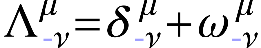

and

, where the infinitesimals

and

are not related to the earlier

and

. Utilizing Equation (1.4.3) and retaining only first-order terms in

and

, Equations (1.4.8) and (1.4.9) simplify to:

By isolating the coefficients of

and

on both sides of these equations, we derive the commutation relations:

In quantum mechanics, particular importance is given to those operators that are conserved, meaning they commute with the energy operator

. A review of Equations (1.4.13) and (1.4.14) reveals that these conserved operators include the momentum three-vector

as well as the energy

itself. The other generators constitute what is termed the 'boost' three-vector

These are not conserved, which is why their eigenvalues are not employed to characterize physical states. Expressed in a three-dimensional notation, the commutation relations (1.4.12), (1.4.13), and (1.4.14) can be represented as:

Here,

take the values 1, 2, and 3, and

is the completely antisymmetric quantity where

. The commutation relation (1.4.18) is identified as belonging to the angular-momentum operator.

The subgroup of pure translations

is a part of the inhomogeneous Lorentz group, and its group multiplication rule, as defined by (1.3.7), is

This multiplication rule is additive, similar to what is described in Equation (1.2.24). Employing Equation (1.4.3) and revisiting the arguments that led to Equation (1.2.26), we determine that finite translations in the physical Hilbert space are represented as

Likewise, a rotation

through an angle

around the direction specified by

is represented in the physical Hilbert space as

Contrasting the Poincaré algebra with the Lie algebra of the Galilean group, the symmetry group for Newtonian mechanics, offers fascinating insights. While it is possible to derive the Galilean algebra beginning with its transformation rules and using the same methodology we used for the Poincaré algebra, a simpler path exists. Since we already possess Eqs. (1.4.18)-(1.4.24), we can more conveniently obtain the Galilean algebra as the Inönü-Wigner contraction of the Poincaré algebra in the low-velocity limit. For a set of particles with an average mass

and velocity

, we anticipate the momentum and angular-momentum operators to be of the order

. On the flip side, the energy operator

is composed of a total mass

and a non-mass energy

(kinetic and potential), which are of the order

. Examining Eqs. (1.4.18)-(1.4.24) reveals that in the limit where

, the commutation relations simplify to:

where

scales as

. It's noteworthy that in Hilbert space, the sequence of operations involving a translation

and a 'boost'

does not yield the expected transformation

. Instead, we have:

The emergence of the phase factor

indicates that we are dealing with a projective representation, which comes with a superselection rule that precludes the mixing of states with different masses. In this aspect, the mathematical framework of the Poincaré group is less complex than that of the Galilean group. Nonetheless, it is entirely feasible to extend the Galilean group formally by introducing an additional generator to its Lie algebra. This new generator would commute with all existing generators and have eigenvalues corresponding to the masses of the different states. In such a scenario, physical states would be represented through an ordinary, rather than projective, representation of the augmented symmetry group. While this might seem like a minor change in notation, it effectively eliminates the necessity for a mass superselection rule within the reinterpreted Galilean group.

We turn our attention to the categorization of single-particle states based on their transformation properties under the inhomogeneous Lorentz group.

Given that the components of the energy-momentum four-vector commute among themselves, it is logical to represent physical state-vectors using eigenvectors of the four-momentum. To do this, we introduce a label

to account for any additional degrees of freedom, leading us to consider state-vectors

such that

For more complex states, like those comprising multiple free particles, the label

would need to accommodate both continuous and discrete values. In this discussion, we are focusing solely on one-particle states, whose definition includes that the label

is purely discrete. It is worth noting that specific bound states of two or more particles, like the ground state of a hydrogen atom, are also considered one-particle states in this context. While such states are not elementary particles, the distinction between composite and elementary particles is irrelevant for our current purposes.

Equations (1.5.1) and (1.4.26) inform us about the transformation behavior of these states under homogeneous Lorentz transformations.

Applying equation (1.4.9), we find that when a quantum homogeneous Lorentz transformation

or equivalently

acts on

, it yields a four-momentum eigenvector with eigenvalue

Generally, one might be able to construct suitable linear combinations of

such that the matrix

becomes block-diagonal. In other words,

with

values within a single block could constitute a representation of the inhomogeneous Lorentz group on their own. It makes sense to associate the states of a particular particle type with components of an irreducible representation of the inhomogeneous Lorentz group, meaning it can't be further broken down in this manner.

It should be noted that different types of particles may be related to isomorphic representations, which means their matrices

could be identical or transformed into one another by a similarity transformation. In certain scenarios, particle types might be defined as irreducible representations of larger groups, which include the inhomogeneous proper orthochronous Lorentz group as a subgroup. For example, for massless particles whose interactions are invariant under space inversion, it's common to treat all components of an irreducible representation of the inhomogeneous Lorentz group as a single particle type.

The next step in our investigation is to elucidate the structure of the coefficients

in irreducible representations of the inhomogeneous Lorentz group.

For our objectives, it's crucial to recognize that the only functions of

left invariant by all proper orthochronous Lorentz transformations

are the invariant square

, and for

, also the sign of

. Therefore, for each specific value of

, and when

, each sign of

, we can select a 'standard' four-momentum denoted as

. Any

within this category can then be represented as

where

is a particular standard Lorentz transformation depending on

and, implicitly, on our chosen standard

. Consequently, the states

having momentum

can be defined as

where

is a numerical normalization factor, the specifics of which will be determined later. Up to this juncture, no details have been provided about how the

labels are connected across varying momenta; Equation (1.5.5) now addresses this absence.

When applying an arbitrary homogeneous Lorentz transformation

to equation (1.5.5), we obtain:

The purpose of this last step is to show that the Lorentz transformation

first maps

, then to

, and finally back to

. This transformation belongs to a subgroup within the homogeneous Lorentz group, characterized by Lorentz transformations

that keep

invariant:

This subgroup is termed the little group. For any

that satisfies Equation (1.5.7), we find that:

The coefficients

serve as a representation of the little group. Specifically, for any elements

the relationship

Aside from normalization issues, the task of identifying the coefficients

in transformation rule (1.5.3) has now been distilled down to finding the representations of the little group. This technique, which involves deriving representations of a larger group like the inhomogeneous Lorentz group from the representations of its little group, is known as the method of induced representations.

	Standard	Little Group
(a)
(b)
(c) ,
(d) ,
(e)
(f)

Table 1.5.1. Standard four-momenta and their associated little groups for different categories of four-momenta are discussed. In this context, represents an arbitrary positive energy, for instance, 1 eV. The little groups are generally straightforward to understand: is the regular three-dimensional rotation group that comprises Lorentz transformations which keep a zero-momentum particle stationary. Meanwhile, and are Lorentz groups in (2+1)-dimensions and (3+1)-dimensions, respectively. The group is the set of transformations in Euclidean geometry, which includes both rotations and translations in two dimensions. Its role as the little group for cases where will be elaborated on later.

Table 1.5.1 provides a suitable selection for the standard four-momentum

along with the associated little group for different categories of four-momenta.

Out of the six categories of four-momenta, only types (a), (c), and (f) have any recognized implications for physical states. For class (f) — where

—it pertains to the vacuum state, which is essentially unchanged by

. Our subsequent discussion will be confined to cases (a) and (c), which correspond to particles with mass

and massless particles, respectively.

Now is an appropriate time to discuss the normalization of these states. Employing the standard orthonormalization procedure from quantum mechanics, we can select states with standard momentum

to be orthonormal as denoted by the equation:

(Let me remark that

is the standard momentum and

runs over all possibilities such that

, so, for example, we can not use (1.5.12) to calculate

. Also

and

are normalized such that (1.5.12) holds) The presence of the delta function arises because

and

are eigenstates of a Hermitian operator with eigenvalues

and

, respectively. As a direct outcome, the representation of the little group in Eqs. (1.5.8) and (1.5.11) must be unitary.

For

and

, the little groups

and

do not possess any non-trivial finite-dimensional unitary representations. Hence, if there were states with a specific momentum

having

that non-trivially transform under the little group, an infinite number of such states would be required.

Regarding the scalar products for generic momenta, the unitarity of the operator

as expressed in Eqs. (1.5.5) and (1.5.11) provides the following formula for the scalar product:

Since

as well, the delta function

is proportional to

. The presence of

implies that only the coefficient when

matters, as otherwise the inner product vanishes. Hence, with

, we have

When integrating an arbitrary scalar function

over four-momenta subject to

and

(corresponding to cases (a) or (c)), the Lorentz-invariant integral takes the form:

Given that

and

are connected to

and

through a Lorentz transformation

, we arrive at the following equation:

The normalization constant

is occasionally set to

. However, in doing so, one would need to account for the

term in scalar products. In this context, we will use the more common convention where:

Next, we turn our attention to the two physically relevant cases: particles with mass

and particles with zero mass.

In this context, the little group is represented by the three-dimensional rotation group. Its unitary representations can be decomposed into a direct sum of irreducible unitary representations, denoted by